Visualizing the definition of continuity

In this first post, I want to focus on a very important definition of real analysis: the continuity of a function. I want to combine both, the formal $\epsilon$ – $\delta$ -definition and a possible visualization of what’s going on and what needs to be done, when showing that a function $f:[a,b]\longrightarrow\mathbb{R}$ is continuous at a point $x\in [a,b]$ . So let’s have a look at the formal definition and a picture that visualizes the statement.

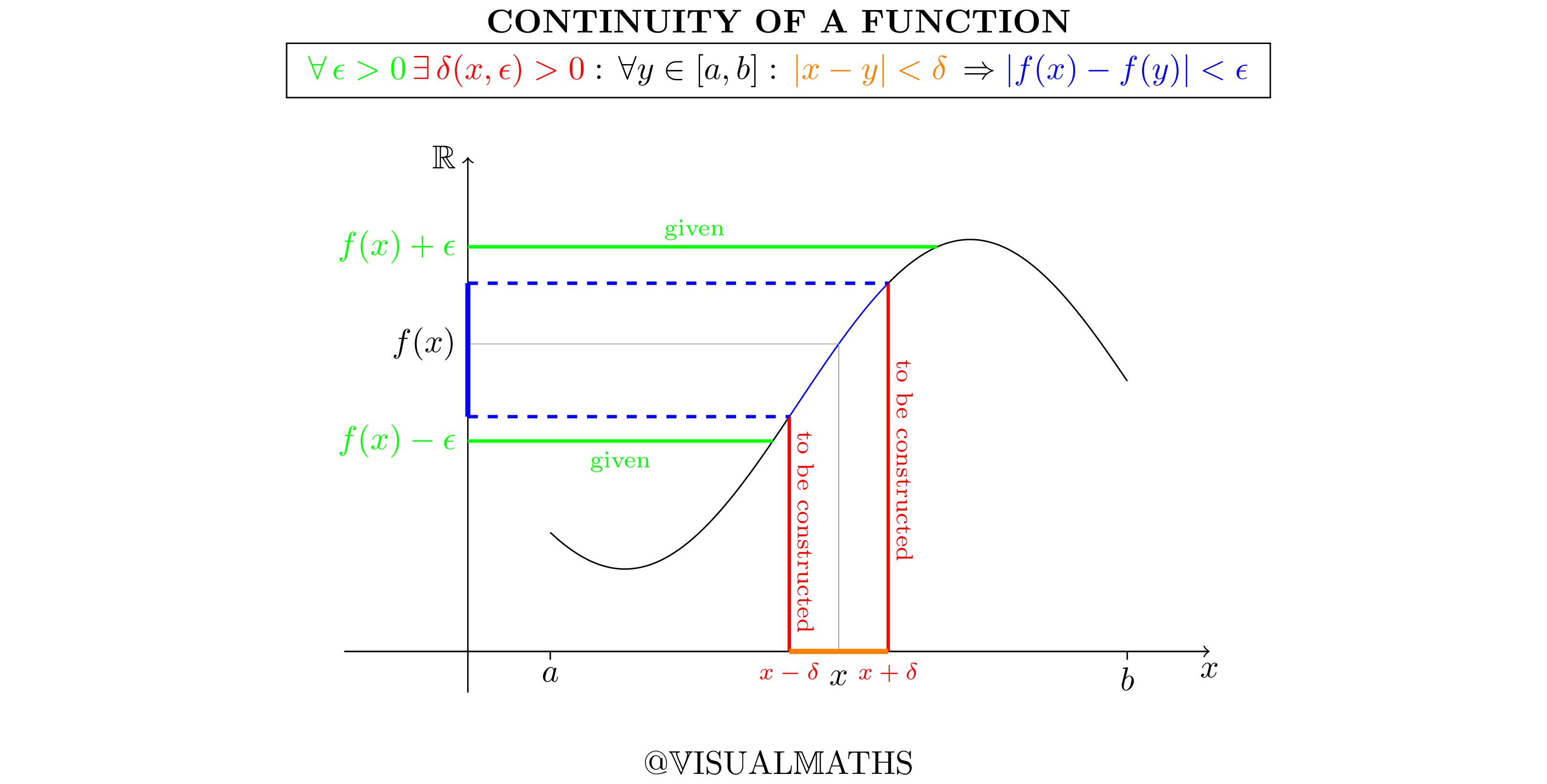
Visualization of the definition of continuity

Let’s repeat the formal definition of continuity at a point $x\in [a,b]$ :

$\forall\epsilon > 0\,\exists\,\delta > 0\text{ such that }\forall y\in [a,b]:\,|x-y|<\delta\,\implies\, |f(x)-f(y)|<\epsilon$

So, what is going on here? Roughly speaking, this definition says that small neighbourhoods around $x\in [a,b]$ get mapped to small neighbourhoods of $f(x)$ . But let’s have a closer look. Without going too deep into predicate logic, it is important to notice that the order of quantors is essential. The first part is that for all (which means, arbitrarily given) $\epsilon > 0$ there exists a $\delta > 0$ . So, what do we need to do? A statement that has to hold for all means, that we cannot put any restrictions on that element. Precise: when proving continuity, we need to whish ourselves an arbitrarily chosen $\epsilon > 0$ , no matter how small or how big it is (see the region enclosed by $f(x)+\epsilon$ and $f(x)-\epsilon$ on the $y$ -axis). From this arbitrary choice, the following existence quantor $\exists$ leads to the next step: we have to show existence! But how do we do that when all we have for the moment is our function $f$ , the point $x\in [a,b]$ and our arbitrary $\epsilon >0$ which doesn’t provide any information? Showing existence means constructing the required element. Precise: we have to construct the $\delta > 0$ from the point $x$ and $\epsilon$ . Note that $\delta$ in general depends on $x$ and $\epsilon$ . Before studying how to construct $\delta$ , let’s go further into the definition. The next part says that all we have done so far has to hold for all $y\in [a,b]$ , that is less far apart than $\delta$ away from $x$ (see the orange region in the picture). So, again: to prove this, we have to chose $y$ arbitrarily. From this, we have to show an implication. This means, that we may assume that $x$ and our arbitrarily chosen $y$ lie less than our constructed $\delta$ away from each other. From this assumption we need to show that our constructed $\delta$ is indeed sufficient to prove $|f(x)-f(y)|<\epsilon$ (see the blue region on the $y$ -axis). And that’s basically it. But: how do we construct $\delta$ ? That’s the tricky part when proving continuity from the definition is the construction because one has to have clever ideas regarding the manipulation of the expression $|f(x)-f(y)|$ . We know by assuming that $|x-y|<\delta$ , so what can we do to make this expression appear in $|f(x)-f(y)|$ ? Yes, try to manipulate until we can estimate by $|x-y|$ , because then we can apply our assumption. Precise:

$\text{Start with }|f(x)-f(y)|=|\text{ insert definition of }f|\leq\ldots$

$\ldots\text{ make clever estimates }\ldots\leq\ldots\leq\ldots$

$\ldots(\text{something with }x)\cdot |x-y|<\delta(x,\epsilon),\text{ by assumption}$

You may ask yourself: why may $\delta$ not depend on $y$ ? The answer is that the existence of $\delta$ in the definition is predicted before saying that the foregoing has to hold for all $y$ .

Let’s have a look at a concrete example: the continuity of $f(x)=x^{2}-x$ .

Let $f:\mathbb{R}\longrightarrow\mathbb{R},\,x\mapsto x^{2}-x$ be given. We want to show that this function is continuous at any $x\in\mathbb{R}$ . Before writing out the formal proof, we have to think about how to get $|x-y|$ into play, starting with $|x^{2}-x-(y^{2}-y)|$ . Notice that the $\delta$ that we are going to choose may only depend on $x$ and $\epsilon$ . So, let’s try to make a clever estimate:

$|f(x)-f(y)|=|x^{2}-x-(y^{2}-y)|=|x^{2}-y^{2}-(x-y)|=|(x-y)(x+y)-(x-y)|=|(x-y)(x+y-1)|=|x-y||x+y-1|\,\,\,(*)$

Fine, so we made it to bring the expression $|x-y|$ into play. The problem is that the rest not only depends on $x$ , but also on $y$ (remember: $\delta$ may not depend on $y$ ). The good news is that we are free to choose any $\delta$ , as long as we can conclude $|f(x)-f(y)|<\epsilon$ . So, let’s make an assumption: let $|y-x|=|x-y|<1=\delta$ . From the reversed triangle inequality we know that $|y|-|x|\leq |y-x|<1 \Leftrightarrow |y|<1+|x|\,\, (**)$ . This is great, since we are now in a position to make an estimate on $y$ in terms of $x$ . So, let’s go ahead and try to make an estimate on $(*)$ :

$|f(x)-f(y)|= \ldots =|x-y||x+y-1|\overset{\triangle \neq}{\leq} |x-y|(|x-1|+|y|) \overset{(**)}{\leq}|x-y|(|x-1|+1+|x|)\overset{\text{by assumption}}{<}\delta (|x-1|+1+|x|)$

Looks good. We’ve made an estimate that does not depend on $y$ and we can now see what our delta has to look like. In order to make the last expression less than $\delta$ , simply take the smaller choice of the two that we made: $\delta:= \text{min}\left(1,\frac{\epsilon}{|x-1|+1+|x|}\right)$ . Now we can wrtite out the formal proof of $f$ being continuous at $x\in[a,b]$ :

Let $\epsilon > 0$ be arbitrarily given. Choose $\delta:= \text{min}\left(1,\frac{\epsilon}{|x-1|+1+|x|}\right)$ . Further, let $y\in [a,b]$ be arbitrary and assume $|x-y|<\delta$ . To show that this choice of $\delta$ implies $|f(x)-f(y)|<\epsilon$ , we make the following estimate:

$|f(x)-f(y)|=|x^{2}-x-(y^{2}-y)|=|x-y||x-1+y|\leq|x-y|(|x-1|+|y|)\leq |x-y|(|x-1|+1+|x|)<\delta(|x-1|+1+|x|)=\frac{\epsilon}{|x-1|+1+|x|}(|x-1|+1+|x|)=\epsilon$

This completes the proof.

Visualizing the definition of continuity

Veröffentlicht von visual maths

Hinterlasse einen Kommentar Antwort abbrechen

Teilen mit:

Ähnliche Beiträge

Veröffentlicht von visual maths

Hinterlasse einen Kommentar Antwort abbrechen